Hunga Tonga Volcanic Eruption & Earth's Ionosphere

This research project was undertaken to fulfill requirements for 'Project 1' of City College of San Francisco's MATH 108 Fundamentals of Data Science course.

• Student: Greg Albrecht W2GMD ionosphere@undef.net
• Instructor: Shawn Wiggins

Introduction to Earth's Ionosphere

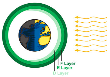
Earth's atmosphere is composed of several layers, each with different physical properties. The ionosphere is region of the atmosphere containing several sub-layers of electrically charged (ionized) gas particles. Depending on the density and energy of these gas particles, radio frequency (RF) traveling through these layers can be absorbed, reflected back to earth, or lost to space.

• Pictured: Ionospheric effects on radio waves at different frequencies.
• Source: NASA https://www.swpc.noaa.gov/phenomena/ionosphere

Sub-layers tend to follow diurnal (day/night) patterns, with E & F being persistent, and D, F1 & F2 emerging only during the day.

• Pictured: Ionosphere layers.
• Source: NWS https://www.weather.gov/jetstream/ionosphere_max

Measuring the Ionosphere

Methods of measuring the properties (sounding) the ionosphere range from active radar-like radio frequency probes to passive GPS satellite signal observation. Ionosonde is the term used for active radio frequency probes.

• Pictured: Ionosonde schematic
• Source: Australian Bureau of Meteorology https://www.planetary.org/space-images/a-basic-schematic-of-an-ionosonde

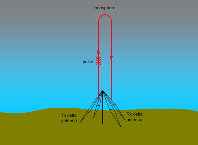
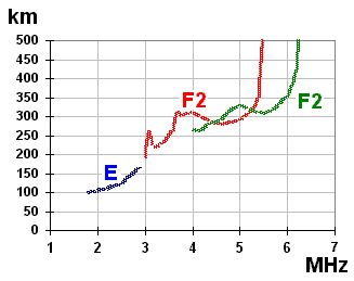
Ionosonde data can be represented visually in the form of an ionogram. Ionograms typically include data such as the Frequency of F2, Frequency of E, Total Electron Content, et al.

• Typical ionogram indicating an F2 layer critical frequency (foF2) of approximately 5.45 MHz.
• Source: Wikipedia https://en.wikipedia.org/wiki/Ionosonde

An international consortium of research institutions runs several ionospheric sounding stations around the planet. These stations probe the ionosphere periodically through the day, year round. This data is used to predict ionospheric conditions that may effect long range radio transmission, satellite signal reception, and global navigation satellite positioning.

• Pictured: Global Ionosphere Radio Observatory (GIRO) Digisonde sites.
• Source: GIRO https://giro.uml.edu/

Heliophysics has the strongest influence on ionospheric conditions, including day/night, solar wind, sun cycles, sun spots, coronal mass ejections (CMEs), et al. Earth weather & geophysics also influence the ionosphere, including weather & storms, tsunamis & earthquakes.

Project Description

• Question: Given the effect of other Earth geophysics on the ionosphere, and our ability to measure ionospheric conditions with some periodicity, can we measure the effects of a volcanic eruption on the ionosphere?

This project aims to use the global ionospheric surveillance network dataset to determine if the Hunga Tonga volcanic eruption in January 2022 had a measurable effect on the ionosphere.

Variables

Variables & measurements we intend to measure include:

• Frequency of F2 (foF2): The highest frequency of radio signal (RF) that would be reflected back to Earth by the F2 layer of the ionosphere. Measured in MHz.
• Total Electron Content (TEC): The total number of electrons present along a path between a radio transmitter and receiver. Measured in 10^16 electrons/m² = 1 TECU

Limitations

Potential limitations to the data used in this project include:

1. The number of stations within range of the volcano. More stations would allow more granular readings.
2. Periodicity is not guaranteed. Ionosonde readings do not appear to be syncronized, and some periods are missing completely.

Future Considerations

• WSPR Data
• CWOP Data
• Space Weather Data

Errata / N.B.

This project originally used raw MIDS data from NOAA, but switched over to use FastChar data from GIRO. Consider all MIDS-related functions DEPRECATED in favor of FastChar.

Sources

The data used in this project comes from these sources:

Ionosonde MIDS & FastChar:

• Reinisch, B. W., and I. A. Galkin, Global ionospheric radio observatory (GIRO), Earth, Planets, and Space, 63, 377-381, doi:10.5047/eps.2011.03.001, 2011.
• http://spase.info/SMWG/Observatory/GIRO
• "This paper uses ionospheric data from the USAF NEXION Digisonde network, the NEXION Program Manager is Annette Parsons"

Other Notes

"A large eruption commenced on 15 January 2022 at 04:20 local time, sending clouds of ash 20 km (12 mi) into the atmosphere."

https://volcano.si.edu/ShowReport.cfm?doi=10.5479/si.GVP.WVAR20220112-243040

https://cimss.ssec.wisc.edu/satellite-blog/archives/44214

https://en.wikipedia.org/wiki/2022_Hunga_Tonga_eruption_and_tsunami

https://appliedsciences.nasa.gov/our-impact/news/tonga-eruption-sent-ripples-through-earths-ionosphere

Look at Guam barometric pressure data to see when pressure wave hit:

https://www.ndbc.noaa.gov/station_history.php?station=aprp7

The 'Code'

Boiler-plate

Imports

# Python standard modules

import datetime
import os
import time
import urllib.request

# CCSF MATH 108 / UCB DATA 8 imports

from datascience import *
import numpy as np

%matplotlib inline
import matplotlib.pyplot as plots
plots.style.use('fivethirtyeight')

# Other external modules used in this notebook

import pandas as pd

Constants

# Into which directories would we save our data:
FASTCHAR_DIR = 'fastchar'
CWOP_DIR = 'cwop'

# If set to True, the following will flush existing data:
FLUSH_FASTCHAR = True
FLUSH_CWOP = False

# Which measurements do we want to retrieve from FastChar?
FASTCHAR_NAMES = 'foF2,foF1,foE,foEs,MUFD,fmin,TEC'

# Hunga Tonga Volcano location:
HUNGA_TONGA_LAT = 20.536
HUNGA_TONGA_LON = 175.382

# When did the eruption start (UTC) January 15, 04:20 UTC
ERUPTION_START = datetime.datetime(2022, 1, 15, 4, 20, tzinfo=datetime.timezone.utc)

Project-specific function definitions

# To access this servlet use format: 
#  DIDBGetValues?ursiCode=CODE&charName=NAME&fromDate=yyyy.mm.dd%20(...)%20hh:mm:ss&toDate=yyyy.mm.dd%20(...)%20hh:mm:ss
# For example: DIDBGetValues?ursiCode=DB049&charName=foF2&fromDate=2007.06.25%20(...)%2000:00:00&toDate=2007.06.26%20(...)%2000:00:00
#  or: DIDBGetValues?ursiCode=DB049&charName=foF2&fromDate=2007.06.25&toDate=2007.06.26

def get_fastchar(usri_code: str) -> str:
    """Downloads FastChar data from the GIRO FastChar API."""
    base_url = 'https://lgdc.uml.edu/common/DIDBGetValues'
    from_date = '2022.01.01'
    to_date = '2022.01.31'
    dmuf = 3000
    url = (f"{base_url}?ursiCode={usri_code}&charName={FASTCHAR_NAMES}"
           f"&fromDate={from_date}&toDate={to_date}&DMUF={dmuf}")
    print(f"Getting FastChar from {url}")

    file_name: str = f"{usri_code}.txt"
    file_path: str = f"{FASTCHAR_DIR}/{file_name}"
    
    # Don't download again
    if os.path.exists(file_path) and not FLUSH_FASTCHAR:
        print(f"FastChar exists: {file_path}")
        return
    try:
        with urllib.request.urlopen(url) as mids_df:
            with open(file_path, "wb+") as mids_file:
                print(f"Saving FastChar to {file_path}")
                mids_file.write(mids_df.read())
        return file_path 
    except Exception as exc:
        print(f"Exception: {exc}")
        return

def calc_dist(lat: float, lon: float) -> float:
    """Calculates distance from Hunga Tonga Volcano."""
    func = haversine_distance
    return func(HUNGA_TONGA_LAT, HUNGA_TONGA_LON, lat, lon)

def fix_ts(ts: str) -> datetime.datetime:
    """Parses the given timestamp as a datetime.datetime in UTC."""
    return datetime.datetime.fromisoformat(f"{ts}+00:00")

def format_fastchar_vals(val):
    """Replaces empty readings (---) with 0 and casts to float."""
    if not isinstance(val, (float, int)):
        return float(val.replace('---', '0'))
    else:
        return val

def download_sleep(inc: int = 20) -> None:
    """Sleeps for a random period to avoid flooding GIRO API."""
    sleep_time = np.random.random() * inc
    print(f"Sleeping for {sleep_time}")
    time.sleep(sleep_time)

def get_cwop(site: str) -> None:
    """Downloads CWOP data from the weather data archive."""
    url: str = f"https://weather.gladstonefamily.net/cgi-bin/wxobservations.pl?days=56&site={site}"
    file_name: str = f"{site}.csv"
    file_path: str = f"{CWOP_DIR}/{file_name}"
    
    # Don't download again
    if os.path.exists(file_path) and not FLUSH_MIDS:
        print(f"CWOP exists: {file_path}")
        return
    
    print(f"Getting CWOP from {url}")
    try:
        with urllib.request.urlopen(url) as mids_df:
            with open(file_path, "wb+") as mids_file:
                print(f"Saving CWOP to {file_path}")
                mids_file.write(mids_df.read())
        return file_path 
    except Exception as exc:
        print(f"Exception: {exc}")
        return

# Cargo-culted radian distance calculation:
def haversine_distance(lat1, lon1, lat2, lon2):
    """
    https://towardsdatascience.com/heres-how-to-calculate-distance-between-2-geolocations-in-python-93ecab5bbba4
    """
    # Earth radius:
    #  Miles: 3959.87433
    #  km: 6372.8
    r = 6372.8

    phi1 = np.radians(lat1)
    phi2 = np.radians(lat2)
    delta_phi = np.radians(lat2 - lat1)
    delta_lambda = np.radians(lon2 - lon1)
    a = np.sin(delta_phi / 2)**2 + np.cos(phi1) * \
        np.cos(phi2) * np.sin(delta_lambda / 2)**2
    res = r * (2 * np.arctan2(np.sqrt(a), np.sqrt(1 - a)))
    return np.round(res, 2)

Data Science!

Create Ionosonde DataTables

station_names = make_array(
    'Pt. Arguello', 
    'Wallops Is.', 
    'Guam', 
    'Learmonth', 
    'Boulder', 
    'Idaho National Lab'
)

usri_codes = make_array(
    'PA836', 
    'WP937', 
    'GU513', 
    'LM42B', 
    'BC840', 
    'IF843'
)

lats = make_array(
    34.80,
    37.90,
    13.62,
    -21.80,
    40.00,
    43.81
)

lons = make_array(
    239.50,
    284.50,
    144.86,
    114.10,
    254.70,
    247.32
)

station_names = Table().with_columns(
    'Name', station_names, 
    'USRI', usri_codes,
)

station_locations = Table().with_columns(
    'USRI', usri_codes,
    'lat', lats,
    'lon', lons 
)
stations = station_names.join('USRI', station_locations, 'USRI')
stations

USRI	Name	lat	lon
BC840	Boulder	40	254.7
GU513	Guam	13.62	144.86
IF843	Idaho National Lab	43.81	247.32
LM42B	Learmonth	-21.8	114.1
PA836	Pt. Arguello	34.8	239.5
WP937	Wallops Is.	37.9	284.5

Data Ingest & Pre-processing

def download_data():
    """Downloads the ionosonde data."""
    if not os.path.exists(FASTCHAR_DIR):
        os.mkdir(FASTCHAR_DIR)

    for usri in stations.column('USRI'):
        print(f"Downloading ionosonde data for {usri=}")
        if get_fastchar(usri):
            download_sleep()

# Only need to run once to download ionosonde data:
# download_data()

def populate_dt():
    """Populates the ionosonde DataTables."""
    main_dt = Table()
    for usri in stations.column('USRI'):
        print(f"Populating DataTable for {usri=}")
        
        # Calculate the distance from Hunga Tonga to the site:
        distance = calc_dist(
            stations.where('USRI', usri).column('lat').item(0),
            stations.where('USRI', usri).column('lon').item(0)
        )

        file_name: str = f"{usri}.txt"
        file_path: str = f"{FASTCHAR_DIR}/{file_name}"

        # Read the 'fixed width' data as a pandas DataFrame,
        #  then convert to a DataTable.            
        station_df = pd.read_csv(
            file_path, 
            sep='\s+',
            skiprows=np.arange(0, 26)
        )
        station_dt = Table().from_df(station_df).relabel('#Time', 'Time')

        # Fix the values for some of our columns:
        station_dt = station_dt\
            .where('foF2', are.not_containing('---'))\
            .where('TEC', are.not_containing('---'))
        
        station_dt = Table().with_columns(
            'ts', station_dt.apply(
                lambda t: datetime.datetime.fromisoformat(t.replace('Z', '+00:00')), 'Time'),
            'foF1', station_dt.apply(format_fastchar_vals, 'foF1'),
            'foF2', station_dt.apply(float, 'foF2'),
            'foE', station_dt.apply(format_fastchar_vals, 'foE'),
            'MUFD', station_dt.apply(format_fastchar_vals, 'MUFD'),
            'fmin', station_dt.apply(format_fastchar_vals, 'fmin'),
            'TEC', station_dt.apply(float, 'TEC'),
            'CS', station_dt.apply(int, 'CS')

        )
        station_dt['USRI'] = usri
        station_dt['Distance'] = float(distance)

        # Append/join this DataTable to the existing DataTable:
        if not main_dt:
            main_dt = station_dt
        else:
            main_dt.append(station_dt)

    # At this point our DataTable should be sanitized. 
    # Return it sorted by Time Stamp.
    return main_dt.sort('ts')

# Populate our DataTable and give us a preview:
main_dt = populate_dt()
main_dt

Populating DataTable for usri='BC840'
Populating DataTable for usri='GU513'
Populating DataTable for usri='IF843'
Populating DataTable for usri='LM42B'
Populating DataTable for usri='PA836'
Populating DataTable for usri='WP937'

ts	foF1	foF2	foE	MUFD	fmin	TEC	CS	USRI	Distance
2022-01-01 00:00:00+00:00	4.45	9.413	3.38	28.16	2	26.3	85	GU513	3329.3
2022-01-01 00:00:00+00:00	0	4.325	0	15.08	1.65	3.9	80	IF843	7018.86
2022-01-01 00:00:00+00:00	0	6.1	0	24.47	2.38	3.4	60	PA836	6406.29
2022-01-01 00:00:08+00:00	0	3.6	0	11.53	1.7	2.6	100	WP937	10179.4
2022-01-01 00:05:08+00:00	0	3.6	0	11.74	1.7	1.8	100	WP937	10179.4
2022-01-01 00:07:30+00:00	0	9.313	3.4	27.38	2	27.3	95	GU513	3329.3
2022-01-01 00:07:30+00:00	0	5.775	0	14.99	3.2	12	90	PA836	6406.29
2022-01-01 00:10:08+00:00	0	3.5	0	11.74	1.7	1.6	100	WP937	10179.4
2022-01-01 00:15:00+00:00	4.7	9.238	3.4	27.27	2	28.9	85	GU513	3329.3
2022-01-01 00:15:00+00:00	0	4.275	0	14.18	1.75	3.7	70	IF843	7018.86

... (30092 rows omitted)

Focus Data

We're going to focus our investigation on the station at Guam.

# Select just one station to focus on:

focus_dt = main_dt.where('USRI', 'GU513')

Visualize Ionosonde Data

Zoomed-out view

For our zoomed-out view we'll look at data for the entire month of January. Red dot represents the eruption.

Scatter: foF2 & TEC

We'll look at two values from the ionosonde, the foF2 and the total electron content (TEC). There is an association between these two values - that is: As the TEC increases so does the foF2.

focus_dt.scatter('foF2', 'TEC')

Line: TEC

The plot below shows TEC measurements for all of January, which seem to follow some diurnal patterns, climaxing during the day and dropping at night.

plots.clf()
plots.figure(figsize = (20, 10))
plots.plot(
    focus_dt.column('ts'), 
    focus_dt.column('TEC'),
    label='TECU'
)
plots.ylabel('Total Electron Content (10^16 m^-2)')
plots.scatter(x=ERUPTION_START, y=np.min(focus_dt.column('TEC')), color='red', zorder=100)
plots.legend()
plots.show()

<Figure size 432x288 with 0 Axes>

Zoomed-in View

To 'zoom-in' we're going to take a snapshot of our data within the day of the eruption.

# Concentrate on a period surrounding the volcanic eruption:
event_start = datetime.datetime(2022, 1, 15, tzinfo=datetime.timezone.utc)
event_end = datetime.datetime(2022, 1, 16, tzinfo=datetime.timezone.utc)

snap_dt = focus_dt.where('ts', are.between(event_start, event_end))
snap_dt

ts	foF1	foF2	foE	MUFD	fmin	TEC	CS	USRI	Distance
2022-01-15 00:00:00+00:00	4.7	7.563	3.2	27.93	2	11.8	95	GU513	3329.3
2022-01-15 00:07:30+00:00	4.47	7.313	3.25	25.1	2	17.6	90	GU513	3329.3
2022-01-15 00:15:00+00:00	0	7.375	3.25	23.61	2	17.1	95	GU513	3329.3
2022-01-15 00:22:30+00:00	0	7.55	3.3	24.85	2.03	16.2	90	GU513	3329.3
2022-01-15 00:30:00+00:00	5	7.688	3.3	24.87	2.03	19.2	95	GU513	3329.3
2022-01-15 00:37:30+00:00	5.1	7.863	3.35	24.82	2	20.5	95	GU513	3329.3
2022-01-15 00:45:00+00:00	0	8.1	3.45	25.24	2.5	20.8	95	GU513	3329.3
2022-01-15 00:52:30+00:00	3.95	8.388	3.33	26.02	2.5	21.7	95	GU513	3329.3
2022-01-15 01:00:00+00:00	5.3	8.613	3.35	26.78	2.38	21.9	95	GU513	3329.3
2022-01-15 01:07:30+00:00	0	8.8	3.53	26.84	2.5	23.8	95	GU513	3329.3

... (134 rows omitted)

Line: TEC

This plot shows the typical diurnal pattern of daytime peak and nightime low, but with a considerable spike shortly after the eruption.

plots.clf()
plots.figure(figsize = (20, 10))
plots.plot(
    snap_dt.column('ts'), 
    snap_dt.column('TEC'),
    label='TECU'
)
plots.ylabel('Total Electron Content (10^16 m^-2)')
plots.xlabel('Time (UTC)')
plots.scatter(x=ERUPTION_START, y=np.min(snap_dt.column('TEC')), color='red', zorder=100)
plots.legend()
plots.show()

<Figure size 432x288 with 0 Axes>

Line: foF2

Similar to the TEC pattern plotted above, the foF2 plot shows usual diurnal pattern, with a notable peak-trough-peak shortly after the eruption, followed by another peak later in the day.

plots.clf()
plots.figure(figsize = (20, 10))
plots.plot(
    snap_dt.column('ts'), 
    snap_dt.column('foF2'),
    label='foF2'
)
plots.ylabel('Frequency of F2 (MHz)')
plots.xlabel('Time (UTC)')
plots.yticks(np.arange(2, 15, step=0.5))
plots.scatter(x=ERUPTION_START, y=np.min(snap_dt.column('foF2')), color='red', zorder=100)
plots.legend()
plots.show()

<Figure size 432x288 with 0 Axes>

Histogram: foF2

This histogram of foF2 shows us the distribution of foF2 readings throughout our snapshot period, with two prominent areas around 2.5 and 10.75 MHz.

snap_fof2 = snap_dt.column('foF2')
snap_bins = np.arange(np.min(snap_fof2), np.max(snap_fof2)+1, .25)
snap_dt.hist('foF2', bins=snap_bins)

Mo' Graphs

Day-over-Day Comparisons: foF2 & TEC

# Create a new DataTable of the day before the eruption
day_before = datetime.timedelta(hours=-24)
day_before_dt = focus_dt.where(
    'ts', 
    are.between(event_start + day_before, event_end + day_before)
)
day_before_dt

ts	foF1	foF2	foE	MUFD	fmin	TEC	CS	USRI	Distance
2022-01-14 00:00:00+00:00	0	10.275	3.42	33.05	2.05	23.6	95	GU513	3329.3
2022-01-14 00:07:30+00:00	0	10.525	3.45	33.49	2	20.4	95	GU513	3329.3
2022-01-14 00:15:00+00:00	0	10.725	3.38	33.62	2.08	30.2	95	GU513	3329.3
2022-01-14 00:22:30+00:00	0	10.75	3.5	33.09	2	33.4	95	GU513	3329.3
2022-01-14 00:30:00+00:00	0	10.75	3.5	32.29	2	35.7	65	GU513	3329.3
2022-01-14 00:52:30+00:00	0	8.9	3.58	28.19	2.03	21.8	35	GU513	3329.3
2022-01-14 01:00:00+00:00	5.03	9.213	3.6	27.67	2.05	25	85	GU513	3329.3
2022-01-14 01:07:30+00:00	4.95	9.013	3.55	26.76	2.1	25.1	90	GU513	3329.3
2022-01-14 01:15:00+00:00	5.03	8.838	3.63	26.38	2.1	25.7	95	GU513	3329.3
2022-01-14 01:22:30+00:00	5.05	8.588	3.53	26.02	2.08	24.5	90	GU513	3329.3

... (164 rows omitted)

day_before_dt.plot('ts', 'TEC')
snap_dt.plot('ts', 'TEC')

Histogram Comparisons: TEC

The following histograms show first the distribution of TEC values for the day proceeding the eruption, followed second by the same measurement for the day of the eruption. Clearly visible on the day of the eruption is the wide range of values, with highs in the 70 TECUs, compared with 40 and below TECUs the day before.

compare_bins = np.arange(0, 80, 10)
day_before_dt.hist('TEC', bins=compare_bins)
snap_dt.hist('TEC', bins=compare_bins)

Larger Line Plots: foF2 & TEC

plots.clf()
plots.figure(figsize = (20, 10))

plots.plot(
    snap_dt.column('ts'), 
    snap_dt.column('foF2'),
    label='foF2',
    color='blue'
)

plots.plot(
    snap_dt.column('ts'), 
    snap_dt.column('TEC'),
    label='TEC',
    color='purple'
)

plots.scatter(x=ERUPTION_START, y=0, color='red', zorder=100)
plots.legend()
plots.show()

<Figure size 432x288 with 0 Axes>

plots.clf()

# We're going to overlay two ionosonde readings,
#  so create two subplots:
fig, ax1 = plots.subplots(figsize = (20, 10))

# Instantiate a second axes that shares the same x-axis:
ax2 = ax1.twinx()

ax1.plot(
    snap_dt.column('ts'), 
    snap_dt.column('foF2'),
    color='blue'
)

ax2.plot(
    snap_dt.column('ts'), 
    snap_dt.column('TEC'),
    color='purple'
)

# Drop a point where the eruption started:
plots.scatter(x=ERUPTION_START, y=0, color="red", zorder=3, label="Eruption start")


ax1.set_title('Digital Ionogram at GU513 Guam')
ax1.set_xlabel('Time (UTC)')
ax1.set_yticks(np.arange(2, 12, step=0.5))
ax1.set_ylabel('Frequency of F2 (MHz)', color='blue')

ax2.set_ylabel('Total Electron Content (10^16 m^-2)', color='purple')

plots.legend()
plots.show()

<Figure size 432x288 with 0 Axes>

Future Considerations: Additional Data Sources

CWOP

Create weather (CWOP) Data Table

# sites = make_array(
#     'AP834', 'E6648', 'F9608', 'C5306',  # Hawai'i
#     'AV797', 'AR312', 'AS176', 'C5988',  # Californi'a
#     'AP204', 'C6723', 'C7496', 'C8539', 
#     'C9585', 'D1970')

# #for site in sites:
# #    get_cwop(site)

Visualize Weather Data

The block below extracts weather data from the CWOP Data Table within the given timespan and renders it as a line plot.

# event_start = datetime.datetime(2022, 1, 15, tzinfo=datetime.timezone.utc)
# event_end = datetime.datetime(2022, 1, 15, 16, tzinfo=datetime.timezone.utc)

# plots.clf()
# plots.figure(figsize = (20, 10))

# for site in sites:
#     cwop_dt = Table().read_table(f"cwop/{site}.csv")
#     cwop_dt = Table().with_columns(
#         'ts', cwop_dt.apply(fix_ts, 'Time (UTC)'),
#         site, cwop_dt.column('Barometric Pressure (mbar)'),
#     )
#     cwop_period_dt = cwop_dt.where('ts', are.between(ERUPTION_START, event_end))
#     plots.plot(
#         cwop_period_dt.column('ts'), 
#         cwop_period_dt.column(site),
#         label=site
#     )
# plots.legend()
# plots.show()

time_to_hit_s = 2 * 60 * 60
time_to_hit_s

7200

# 5833872
dist_to_hit_m = 3328.36 * 1000
dist_to_hit_m

3328360.0

dist_to_hit_m / time_to_hit_s

462.27222222222224

# Gets the graphics displayed below, only need to run once:
# !wget https://giro.uml.edu/common/img/giro-map-large.gif
# !wget https://www.swpc.noaa.gov/sites/default/files/styles/medium/public/Ionosphere.gif
# !wget https://www.weather.gov/images/jetstream/atmos/ionlayers.jpg
# !wget https://planetary.s3.amazonaws.com/web/assets/pictures/20170815_ionosonde.png
# !wget https://upload.wikimedia.org/wikipedia/commons/6/69/Ionogramme.png